Stop guessing, use data! (Or how we estimate at Lunar Logic)
In our line of business estimating software projects is our bread and butter. Sometimes it’s the first thing our potential clients ask for. Sometimes we have already finished a product discovery workshop before we talk about it. Sometimes it is a recurring task in projects we run.
Either way, the goal is always the same. A client wants to know how much time building a project or a feature set is going to take and how costly it will be. It is something that heavily affects all planning activities, especially for new products, or even defines the feasibility of a project.
In short, I don’t want to discuss whether we need to estimate. I want to offer an argument how we do it and why. Let me, however, start with how we don’t do estimation.
Expert Guess
The most common pattern that we see when it comes to estimation is the expert guess. We ask people who would be doing work how long a task will take. This pattern is used when we ask people about hours or days, but it is also in work when we use story points or T-shirt sizes.
After all, saying a task will take 8 hours is an uncertain assessment as much as saying that it is 3 story point task or it is an S size. The only difference is the scale we are using.
The key word here is uncertainty. We make our expert guesses in the area of huge uncertainty. When I offer that argument in discussions with our clients typically the visceral reaction is “let’s add some details to the scope of work so we understand tasks better.”
Interestingly, making more information available to estimators doesn’t improve the quality of estimates, even if it improves the confidence of estimators. In other words, a belief that adding more details to the scope makes an estimate better is a myth. The only outcome is that we feel more certain about the estimate even if it is of equal or worse quality.
The same observation is true when the strategy is to split the scope into finer-grained tasks. It is, in a way, adding more information. After all, to scope finer-grained tasks out we need to make more assumptions. If not for anything else we do that to define boundaries between smaller chunks. Most likely we wouldn’t stop there but also attempt to keep the level of details we’ve had in the original tasks, which means even more new assumptions.
Another point that I often hear in this context is that experience in estimating helps significantly in providing better assessments. The planning fallacy described by Roger Buehler shows that this assumption is not true either. It also pinpoints that having a lot of expertise in the domain doesn’t help nearly as much as we would expect.
Dan Kahneman in his profound book Thinking Fast and Slow argues that awareness of our flaws in the thinking process doesn’t protect us from falling into the same trap over again. It means that even if we are aware of our cognitive biases we are still vulnerable to them when making a decision. By the same token, simple awareness that expert guess as an estimation technique failed us many times before and knowledge why it was so, doesn’t help us to improve our estimation skills.
That’s why we avoid expert guesses as a way to estimate work. We use the technique on rare occasions when we don’t have any relevant historical data to compare. Even then we tend to do it at a very coarse-grained level, e.g. asking ourselves how much we think the whole project would take, as opposed to assessing individual features.
Ultimately, if expert guess-based estimation doesn’t provide valuable information there’s no point in spending time doing it. And we are talking about activities that can take as much as a few days of work for a team each time we do it. That time might have been used to actually build something instead.
Story Points
While I think of expert guesses as a general pattern, one of its implementations–story point estimation–deserves a special comment. There are two reasons for that. One is that the technique is widely-spread. Another is that there seems to be a big misconception of how much value story points provide.
The initial observation behind introducing story points as an estimation scale is that people are fairly good when it comes to comparing the size of tasks even if they fail to figure out how much time each of the tasks would take exactly. Thanks to that, we could use an artificial scale to say that one thing is bigger than the other, etc. Later on, we can figure out how many points we can accomplish in a cadence (or a time box, sprint, iteration, etc., which are specific implementations of cadences).
The thing is that it is not the size of tasks but flow efficiency that is a crucial parameter that defines the pace of work.
For each task that is being worked on we can distinguish between work time and wait time. Work time is when someone actively works on a task. Wait time is when a task waits for someone to pick it up. For example, a typical task would wait between coding and code review, code review and testing, and so on and so forth. However, that is not all. Even if a task is assigned to someone it doesn’t mean that it is being worked on. Think of a situation when a developer has 4 tasks assigned. Do they work on all of them at the same time? No. Most likely one task is active and the other three are waiting.
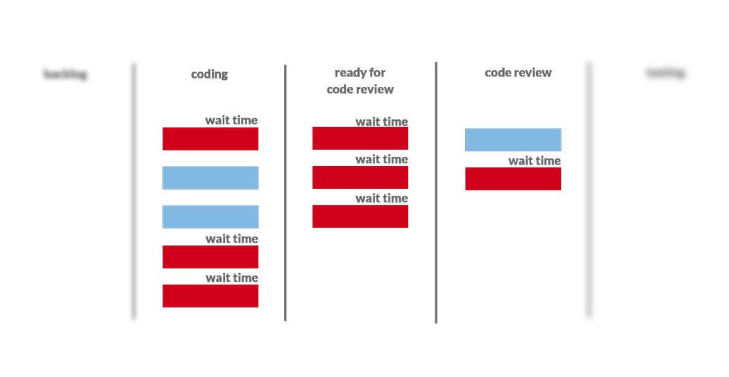
The important part about flow efficiency is that, in the vast majority of cases, wait times outweigh work time heavily. Flow efficiency of 20% is considered normal. This means that a task waits 4 times as much as it’s being worked on. Flow efficiency as low as 5% is not considered rare. It translates to wait time being 20 times longer than work time.
With low flow efficiency, doubling the size of a task will contribute only to a marginal change in the total time that the task spends in the workflow (lead time). With 15% flow efficiency and doubling the size of the task lead time would be only 15% longer than initially. Tripling the size of the task would only result in a lead time that is 30% longer. Let me rephrase: we just increased the size of the task three times and the impact on lead time is less than one third of what we had initially.

Note, I go by the assumption that increasing the size of a task wouldn’t result in increased wait time. Rarely, if ever, such an assumption would hold true.
This observation would lead to a conclusion that investing time into any sizing activity, be it a story point estimation or T-shirt sizing, is not time well-invested. It has been, as a matter of fact, confirmed by the research run by Larry Maccherone, who gathered data from ten thousand agile teams. One of the findings that Larry reported was that velocity (story points completed in a time box) is not any better than throughput (a number of stories completed in a time frame).
In other words, we don’t need to worry about the size of tasks, stories or features. It is enough to know the total number of them and that’s all we need to understand how much work there is to be done.
The same experience is frequently reported by practitioners, and here’s one example.
If there is value in any sizing exercise, be it planning poker or anything else, it is in two cases. We either realize that a task is simply too big when compared to others or we have no clue what a task is all about.
We see this a lot when we join our clients in more formalized approaches to sizing. If there is any signal that we get from the exercise it is when the biggest size that is in use is used (“too big”) or a team can’t tell, even roughly, what the size would be (“no clue”). That’s by the way what inspired these estimation cards.
Historical Data
If we avoid expert guesses as an estimation strategy what other options do we have? There is a post on how approaches to estimation evolved in the agile world and I don’t want to repeat it here in full.
We can take a brief look, however, at the options we have. The approaches that are available basically fall into two camps. One is based on expert guess and I focused on that part in the sections above. The other one is based on historical data.
Why do we believe the latter is superior? As we already established we, as humans, are not well-suited to estimate. Even when we are aware that things went wrong in the past we tend to assume optimistic scenarios for the future. We forget about all the screw-ups we fought, all the rework we did, and all the issues we encountered. We also tend to think of ideal hours, despite the fact that we don’t spend 8 hours a day at our desks. We attend meetings, have coffee breaks, play fussball matches, and chat with colleagues. Historical data remembers it all since all these things affect lead times, and throughput.
Lead time for a finished task would also include the additional day when we fought a test server malfunction, a bank holiday that happened at that time, and unexpected integration issue we found when working on a task. We would be lucky if our memory remembered one of these facts.
By the way, I had the opportunity to measure what we call active work time in a bunch of different teams in different organizations. We defined active work time as time actively spent on doing work that moves tasks from a visual board towards completion when compared to the whole time of availability of team members. For example, we wouldn’t count general meetings as active work time but a discussion about a feature would fall into this category. To stick with the context of this article, we wouldn’t count estimation as active work time.
Almost universally I was getting active work time per team in a range of 30%-40%. This shows how far from the ideal 8-hour long workday we really are despite our perceptions. And it’s not the fact that these teams were mediocre. Conversely, many of them were considered top performing teams in their organizations.
Again, looking at historical lead times for tasks we would have the fact that we’re not actively working 8 hours a day taken care of. The best part is that we don’t even need to know what our active work time is.
Throughput
The simplest way of exploiting historical data is looking at throughput. In a similar manner we account for velocity we may get the data about throughput in consecutive time boxes. Once we have a few data points we may provide a fairly certain forecast what can happen within the next time box.
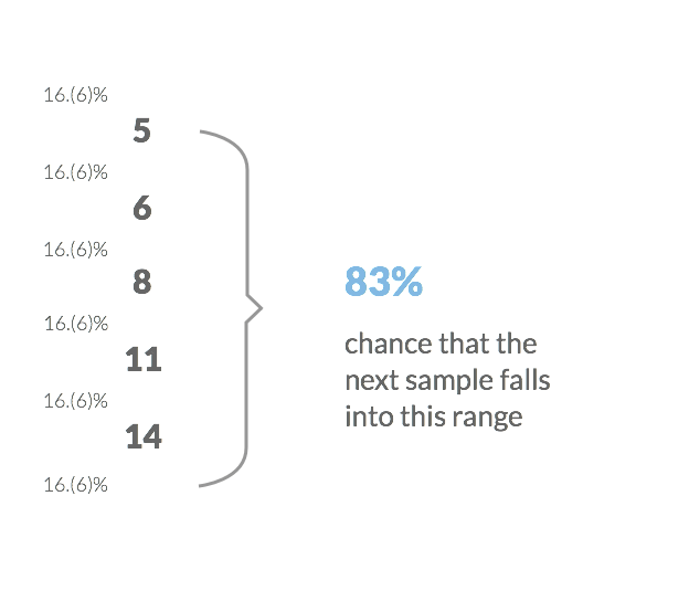
Let’s say that in 5 consecutive iterations there has been 8, 5, 11, 6 and 14 stories delivered respectively. On one hand, we know that we have a range of possible throughput values at least as wide as 5 to 14. However, we can also say that there’s 83% probability that in the next sprint we will finish at least 5 stories (in this presentation you can find the full argument why). We are now talking about a fairly high probability.
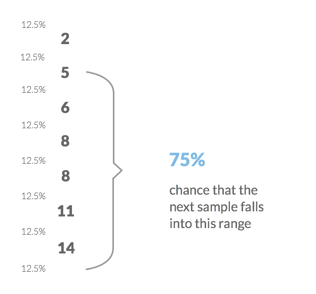
And we had only five data points. The more we have the better we get with our predictions. Let’s assume that in the next two time boxes we finished 2 and 8 stories respectively. Pretty bad result, isn’t it? However, if we’re happy with the confidence level of our estimate around 80% we would again say that in the next iteration we would most likely finish at least 5 stories (this time there’s 75% probability). It is true, despite the fact that we’ve had a couple pretty unproductive iterations.
Note, in this example I ignore completely the size of the tasks. One part of the argument why is provided above. Another part is that we can fairly safely assume that tasks of different sizes would be distributed across different time boxes so we are actually invisibly taking size into consideration.
The best part is that we don’t even need to know the exact impact of the size of a task on its lead time and, as a result, throughput. Yet again, it is taken care of.
Delivery Rate
Another neat way of using historical data is delivery rate, which is based on the idea of takt time. In manufacturing takt time presents how frequently manufacturing of an item is started (or finished). Using it we can figure out throughput of a production line.
In software development, workflow is not as predictable and stable as in manufacturing. Thus, when I talk about delivery rate, I talk about average numbers. Simply put, in a stable context, i.e. stable team setup, in the longer time frame we divide the time (number of days) by a number of delivered features. The answer we’d get would be how frequently, on average, we deliver new features.
We can track different time boxes, e.g. iterations, different projects, etc., to gather more data points for analysis. Ideally, we would have a distribution of possible delivery rates in different team lineups.
Now, to assess how much time a project would take all we need is a couple of assumptions: how many features we would eventually build and what team would work on the project. Then we can look at the distribution of delivery rates for projects built by similar teams, pick data points for the optimistic and pessimistic boundaries and multiply it by the number of features.
Here’s a real example from Lunar Logic. For a specific team setup, we had delivery rate between 1.1 and 1.65 days. It means that a project which we think will have 40-50 features would take between 44 (1.1 x 40) and 83 (1.65 x 50) days.
Probabilistic Simulation
The last approach described above, technically speaking, is oversimplified, incorrect even, from a mathematical perspective. The reason is that we can’t use averages if the data doesn’t follow normal distribution. However, from our experience the outcomes it produces, even if not mathematically correct, are of quality high enough. After all with estimation we don’t aim to be perfect; we just want to be significantly better than what expert guesses provide.
By the same token, if we use a simplified version of throughput-based approach and just go with an average throughput to assess the project the computation wouldn’t be mathematically correct either. Yet still, it would most likely be better than expert guesses.
We can improve both methods and make them mathematically correct at the same time. The technique we would use for that is the Monte Carlo simulation. Put simply, it means that we randomly choose one data point from the pool of available samples and assume it will happen again in a project we are trying to assess.
Then we run thousands and thousands of such simulations and we get a distribution of possible outcomes. Let me explain it basing on the example with throughput we’ve used before.
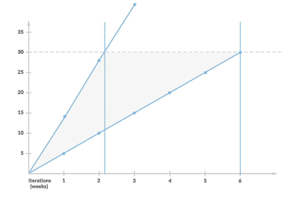
Historically, we had a throughput of 8, 5, 11, 6 and 14. We still have 30 stories to finish. We randomly pick one of data samples. Let’s say it was 11. Then we do it again. We keep picking until the sum of picked throughputs reach 30 (as this is how much work is left to be done). The next picks are 5, 5 and 14. At this time we stop a single run of simulation assessing that remaining work requires almost 4 iterations more.
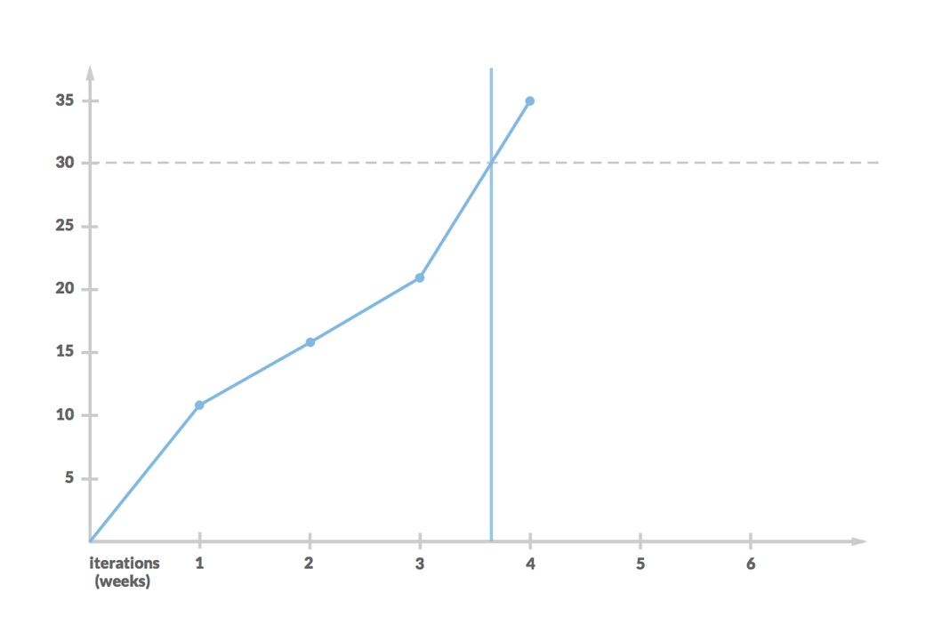
It is easy to understand when we look at the outcome of the run in a burn-up chart. It neatly shows that it is, indeed, a simulation of what can really happen in future.
Now we run such a simulation, say, ten thousand times. And we get a distribution of the results between a little bit more than 2 iterations (the most optimistic boundary) up to 6 iterations (the most pessimistic boundary). By the way, both extremes are highly unlikely. Looking at the whole distribution we can find an estimate for any confidence level we want.
We can adopt the same approach and improve delivery rate technique. This time we would use a different randomly picked historical delivery rate for each story we assess.
Oh, and I know that “Monte Carlo method” sounds scary, but the whole computation can be done in excel sheet with super basic technical skills. There’s no black magic here whatsoever.
Statistical Forecasting
Since we have already reached the point when we know how to employ the Monte Carlo simulation we can improve the technique further. Instead of using oversimplified measures, such as throughput or delivery rate, we can run a more comprehensive simulation. This time, we are going to need lead times (how much time has elapsed since we started a task till we finished it) and Work in Progress (how many ongoing tasks we’ve had during a day) for each day.
The simulation is somewhat more complex this time as we look at two dimensions: how many tasks are worked on each day and how many days each of those tasks takes to complete. The mechanism, though, is exactly the same. We randomly choose values out of historical data samples and run the simulation thousands and thousands of times.
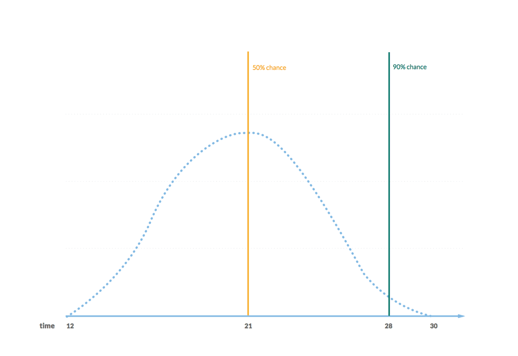
At the end, we land with a distribution of possible futures and for each confidence level we want we can get a date when the work should be completed.
The description I’ve provided here is a super simple version of what you can find in the original Troy Magennis’ work. For doing that kind of simulation one may need to employ support of software tools.
As a matter of fact, we have an early version of a tool developed at Lunar Logic that helps us to deal with statistical forecasting. Projectr (as this is the name of the app) can be fed with anonymized historical data points and the number of features and it produces a range of forecasts for different confidence levels.
To make things as simple as possible we only need start and finish dates for each task we feed Projectr with. This is in perfect alignment with my argument above that size of tasks in the vast majority of cases is negligible.
Estimation at Lunar Logic
I already provided you with plenty of options how estimation may be approached. However, I started with a premise of sharing how we do that at Lunar Logic. There have been hints here and there in the article, but the following is a comprehensive summary.
There are two general cases when we get asked about estimates. First, when we are in the middle of a project and need to figure out how much time another batch of work or the remaining work is going to take. Second, where we need to assess a completely new endeavor so that a client can get some insight about budgetary and timing constraints.
The first case is a no-brainer for us. In this case, we have relevant historical data points in the context that interests us (same project, same team, same type of tasks, etc.). We simply use statistical forecasting and feed the simulation with the data from the same project. In fact, in this scenario we also typically have pretty good insight into how firm our assumptions about the remaining scope of work are. In other words, we can fairly confidently tell how many features, stories or tasks there is to be done.
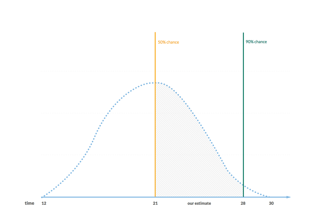
The outcome is a set of dates along with confidence levels. We would normally use a range of confidence levels 50% (half the time we should be good) to 90% (9 times out of 10 we should be good). The dates that match the confidence levels of 50% and 90% serve as our time estimate. That’s all.
The second case is trickier. In this case, we first need to make an assumption about the number of features that constitutes the scope of a project. Sometimes we get that specified from a client. Nevertheless, our preferred way of doing this is to go through what we call a discovery workshop. One of the outcomes of such a workshop is a list of features of a granularity that is common for our projects. This is the initial scope of work and the subject for estimation.
Once we have that, we need to make an assessment about the team setup. After all, a team of 5 developers supported with a full-time designer and a full-time tester would have different pace that a team of 2 developers, a part-time designer and a part-time tester. Note: it doesn’t have to be the exact team setup that will end up working on the project but ideally it is as close to that as possible.
When we have made explicit assumptions about team setup and a number of features then we look for past projects that had a similar team setup and roughly the same granularity of features. We use the data points from these projects to feed the statistical forecasting machinery.
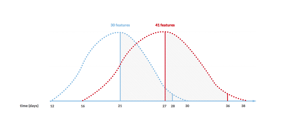
Note: I do mention multiple projects as we would run the simulation against different sets of data. This would yield a broader range of estimated dates. The most optimistic end would refer to 50% confidence level in the fastest project we used in the simulation. The most pessimistic end would refer to 90% confidence level in the slowest project we used in the simulation.
In this case, we still face a lot of uncertainty, as the most fragile part of the process are the assumptions about the eventual scope, i.e. how many features we would end up building.
In both cases, we use statistical forecasting as the main method of estimation. Why would I care to describe all other approaches then? Well, we do have them in our toolbox and use them too, although not that frequently.
We sometimes use a simple assessment using delivery rate (without the Monte Carlo simulation) as a sanity check whether the outcomes of our statistical forecast aren’t off the chart. On occasions we even retreat back to expert guess, especially in projects that are experimental.
One example would be a project in a completely new technology. In this kind of situation the amount of technical research and discovery would be significant enough that would make forecasting unreliable. However, even on such occasions we avoid sizing or making individual estimates for each task. We try to very roughly assess the size of the whole project.
We use a simple scale for that: can it be accomplished in hours, days, weeks, months, quarters or years? We don’t aim to answer “how many weeks” but rather figure out what order of magnitude we are talking about. After all, in a situation like that we face a huge amount of uncertainty so making a precise estimate would only mean that we are fooling ourselves.
This is it. If you went through the whole article you know exactly what you can expect from us when you ask us for an estimate. You also know why there is no simple answer to a question about estimation.
